Primes and self-similarity

Song: John Hollenbeck & NDR Big Band, "Entitlement"
I've been messing around with prime numbers, because there are several places where they intersect with both random walks and the arcsine distribution. It's going to take a while to finally tie that bow, though.
So it's a quick one this week: a kinda-cool story, and a kinda-cool graph.
Random Primes
The prime numbers are simple to find, but not easy. They're not randomly distributed, but it's hard to come up with easy ways to find them, and they act like random numbers in certain ways. Why is 47 prime and 57 non-prime? You can't really tell just by looking.
To find the primes, we can write down every number from, say, 1 to 1000. Then we cross out 2, and every number divisible by 2 (4, 6, 8, etc.). Repeat that with 3 (6, 9, 12, etc.), and so on. The numbers left behind are prime. This is the famous Sieve of Eratosthenes -- it's a tedious way to find prime numbers, but it's by far the easiest to understand.
The sieve gave mathematician David Hawkins an idea [1]: what about doing that same process, but randomly? For each number, flip a coin, if it comes up heads, cross the number out. That will eliminate half of the numbers on the first pass. Take the lowest number k that remains and eliminate each of the remaining numbers with probability 1/k. Say it's 4. For each remaining number, we flip a 4 sided die and if it comes up 4, we cross it out.
If we go through all the numbers, what's left over won't look like real prime numbers -- there should be as many even fake primes as odd ones, for starters. But the remaining numbers will be as sparse as the actual prime numbers. As the sample size N heads to infinity, the chances of a random number being a real prime, and being a fake prime, are the same -- 1/log(N).
This is a brilliant way to figure out what we know about prime numbers are due to their density, and what are due to other, seemingly more magical (but still non-random) factors.
Several characteristics of real primes apply to the random primes. And tantalizingly, things that can't be proven about real primes can be proven about the fake ones. It's been conjectured that there are infinitely many pairs of twin primes -- primes that are separated by 2 numbers. An example would be 5 and 7, or 11 and 13. It makes sense for a lot of reasons that there should be an infinite number of twin primes. But mathematicians have been trying to prove it for over 150 years, without success.
Random primes can be odd or even, so the analogy to twin primes would be two random primes that are only one apart, say 5 and 6. It's relatively simple to prove that there are an infinite number of random twin primes [2]. That could easily be fool's gold -- treating the primes like they're randomly distributed gives mathematicians a whole toolbox of statistical techniques to use on them, but they're not random, or arbitrary. They're perfectly logical, and yet still inscrutible, hidden in plain sight.
Largest prime factors of composite numbers
I was intrigued by the largest prime factor of composite (non-prime) numbers. Are there any patterns?
As background, every number can be split into a unique set of prime factors. For instance, the number 24 can be factored into 24 = 8 * 3 = 2 * 2 * 2 * 3. Let's say we knock off the biggest prime factor. We get: 2 * 2 * 2 = 8. The raw numbers rapidly get too big, so I looked at the log of the ratio:
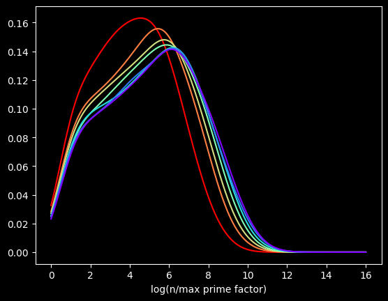
The red curve is the distribution of the first 100,000 composite numbers, the orange is the next 100,000 composite numbers, and so on.
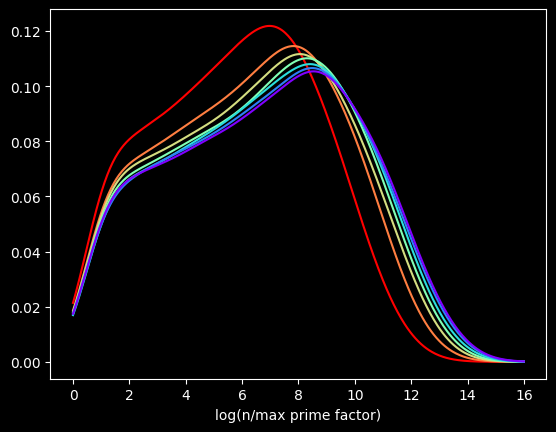
What if we bump up an order of magnitude? This time, the red curve is the first million composite numbers, the orange is the next million, and so on. Here's what that looks like:

Pretty much the same graph, right? The X axis is different, but the shapes are very similar to the first one.
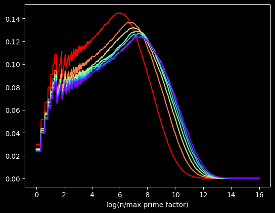
Let's go another order of magnitude up. The first 10,000,000 versus the next 10,000,000, and so on?
We get the same basic shapes again! The self-similarity is kinda cool. Is it possible to come up with some function for the distribution for this quantity? You tell me.
The perils of interpolation
These graphs are flawed. I'm generating these graphs using Kernel Density Estimation, a technique for visualizing the density of data. Histograms, another common way, can be misleading. The choice of bin size can radically alter what the histogram looks like.
But KDE can also be misleading. These graphs make it look like the curve starts at zero. That's not true. The minimum possible value happens when a number is of the form 2*p, where p is a prime -- the value will be log(2), about .693.
This data is actually way chunkier than KDE is treating it. Every point of data is the log of a whole number. So there aren't that many unique values. For instance, between 0 and 1 on the X axis, there's only one possible value -- log(2). Between 1 and 3, there are only 18 possible values, log(2) thru log(19) -- those being the only integers with a log less than 3 and greater than 1.
This makes it hard to visualize the data accurately. There are too many possible values to display each one individually, but not enough for KDE's smoothing to be appropriate.
The kernel in Kernel Density Estimation is the algorithm used to smooth the data -- it's basically a moving average that assumes something about the distribution of the data. People usually use the Gaussian kernel, which treats the data like a normal distribution -- smooth and bell curvy. A better choice for chunky data is the tophat kernel, which treats the space between points like a uniform distribution -- in other words, a flat line. If the sparseness of the data on the X axis were due to a small sample size, the tophat kernel would display plateaus that aren't in the real data. But here, I calculated data for the first 100 Million numbers, so there's no lack of data. The sparseness of the data is by construction. log(2) will be the only value between 0 and 1, no matter how many numbers we go up to. So the left side of the graph should look fairly chunky.
The tophat kernel does a much better job of conveying the non-smoothness of the distribution:
References
[1] https://chance.dartmouth.edu/chance_news/recent_news/chance_primes_chapter2.html
[2] for sufficiently large values of simple
[3] https://scikit-learn.org/stable/auto_examples/neighbors/plot_kde_1d.html
[4] https://en.wikipedia.org/wiki/Kernel_density_estimation