Sep 23, 2025

Song: John Hollenbeck & NDR Big Band, "Entitlement"
I've been messing around with prime numbers, because there are several places where they intersect with both random walks and the arcsine distribution. It's going to take a while to finally tie that bow, though.
So it's a quick one this week: a kinda-cool story, and a kinda-cool graph.
Random Primes
The prime numbers are simple to find, but not easy. They're not randomly distributed, but it's hard to come up with easy ways to find them, and they act like random numbers in certain ways. Why is 47 prime and 57 non-prime? You can't really tell just by looking.
To find the primes, we can write down every number from, say, 1 to 1000. Then we cross out 2, and every number divisible by 2 (4, 6, 8, etc.). Repeat that with 3 (6, 9, 12, etc.), and so on. The numbers left behind are prime. This is the famous Sieve of Eratosthenes -- it's a tedious way to find prime numbers, but it's by far the easiest to understand.
The sieve gave mathematician David Hawkins an idea [1]: what about doing that same process, but randomly? For each number, flip a coin, if it comes up heads, cross the number out. That will eliminate half of the numbers on the first pass. Take the lowest number k that remains and eliminate each of the remaining numbers with probability 1/k. Say it's 4. For each remaining number, we flip a 4 sided die and if it comes up 4, we cross it out.
If we go through all the numbers, what's left over won't look like real prime numbers -- there should be as many even fake primes as odd ones, for starters. But the remaining numbers will be as sparse as the actual prime numbers. As the sample size N heads to infinity, the chances of a random number being a real prime, and being a fake prime, are the same -- 1/log(N).
This is a brilliant way to figure out what we know about prime numbers are due to their density, and what are due to other, seemingly more magical (but still non-random) factors.
Several characteristics of real primes apply to the random primes. And tantalizingly, things that can't be proven about real primes can be proven about the fake ones. It's been conjectured that there are infinitely many pairs of twin primes -- primes that are separated by 2 numbers. An example would be 5 and 7, or 11 and 13. It makes sense for a lot of reasons that there should be an infinite number of twin primes. But mathematicians have been trying to prove it for over 150 years, without success.
Random primes can be odd or even, so the analogy to twin primes would be two random primes that are only one apart, say 5 and 6. It's relatively simple to prove that there are an infinite number of random twin primes [2]. That could easily be fool's gold -- treating the primes like they're randomly distributed gives mathematicians a whole toolbox of statistical techniques to use on them, but they're not random, or arbitrary. They're perfectly logical, and yet still inscrutible, hidden in plain sight.
Largest prime factors of composite numbers
I was intrigued by the largest prime factor of composite (non-prime) numbers. Are there any patterns?
As background, every number can be split into a unique set of prime factors. For instance, the number 24 can be factored into 24 = 8 * 3 = 2 * 2 * 2 * 3. Let's say we knock off the biggest prime factor. We get: 2 * 2 * 2 = 8. The raw numbers rapidly get too big, so I looked at the log of the ratio:
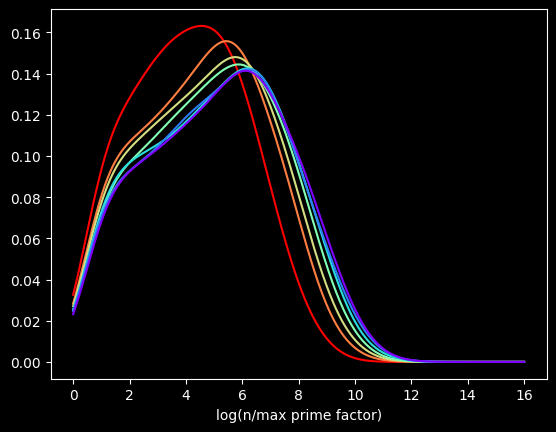
The red curve is the distribution of the first 100,000 composite numbers, the orange is the next 100,000 composite numbers, and so on.
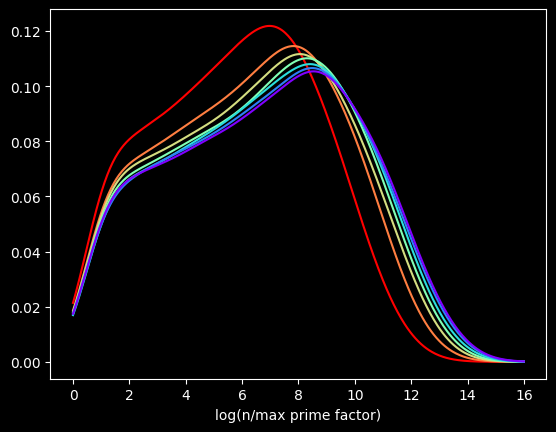
What if we bump up an order of magnitude? This time, the red curve is the first million composite numbers, the orange is the next million, and so on. Here's what that looks like:

Pretty much the same graph, right? The X axis is different, but the shapes are very similar to the first one.
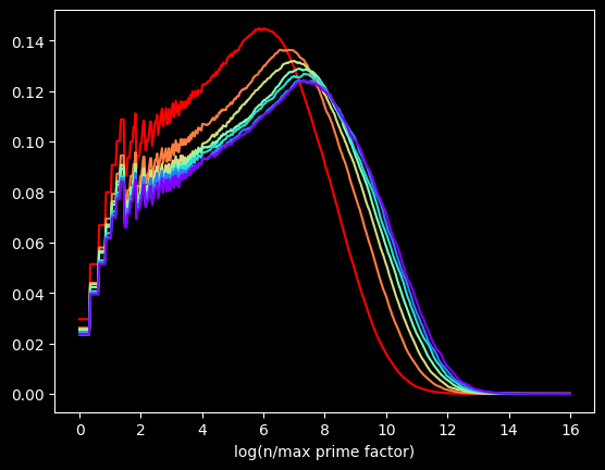
Let's go another order of magnitude up. The first 10,000,000 versus the next 10,000,000, and so on?
We get the same basic shapes again! The self-similarity is kinda cool. Is it possible to come up with some function for the distribution for this quantity? You tell me.
The perils of interpolation
These graphs are flawed. I'm generating these graphs using Kernel Density Estimation, a technique for visualizing the density of data. Histograms, another common way, can be misleading. The choice of bin size can radically alter what the histogram looks like.
But KDE can also be misleading. These graphs make it look like the curve starts at zero. That's not true. The minimum possible value happens when a number is of the form 2*p, where p is a prime -- the value will be log(2), about .693.
This data is actually way chunkier than KDE is treating it. Every point of data is the log of a whole number. So there aren't that many unique values. For instance, between 0 and 1 on the X axis, there's only one possible value -- log(2). Between 1 and 3, there are only 18 possible values, log(2) thru log(19) -- those being the only integers with a log less than 3 and greater than 1.
This makes it hard to visualize the data accurately. There are too many possible values to display each one individually, but not enough for KDE's smoothing to be appropriate.
The kernel in Kernel Density Estimation is the algorithm used to smooth the data -- it's basically a moving average that assumes something about the distribution of the data. People usually use the Gaussian kernel, which treats the data like a normal distribution -- smooth and bell curvy. A better choice for chunky data is the tophat kernel, which treats the space between points like a uniform distribution -- in other words, a flat line. If the sparseness of the data on the X axis were due to a small sample size, the tophat kernel would display plateaus that aren't in the real data. But here, I calculated data for the first 100 Million numbers, so there's no lack of data. The sparseness of the data is by construction. log(2) will be the only value between 0 and 1, no matter how many numbers we go up to. So the left side of the graph should look fairly chunky.
The tophat kernel does a much better job of conveying the non-smoothness of the distribution:
References
[1] https://chance.dartmouth.edu/chance_news/recent_news/chance_primes_chapter2.html
[2] for sufficiently large values of simple
[3] https://scikit-learn.org/stable/auto_examples/neighbors/plot_kde_1d.html
[4] https://en.wikipedia.org/wiki/Kernel_density_estimation
Sep 10, 2025

Song: Klonhertz, "Three Girl Rhumba"
Notebook available here
Think of a number
Pick a number between 1-100.
Say I write down the numbers from 1-100 on pieces of paper and put them in a big bag, and randomly select from them. After every selection, I put the paper back in the bag, so the same number can get picked more than once. If I do that 100 times, what is the chance of your number being chosen?
The math isn't too tricky. It's often easier to calculate the chances of a thing not happening, then subtract that from 1, to get the chances of the thing happening. There's a 99/100 chance your number doesn't get picked each time. So the probability of never getting selected is $(99/100)^{100} = .366$. Subtract that from one, and there's a 63.4% chance your number will be chosen. Alternately, we'd expect to get 634 unique numbers in 1000 selections.
When I start picking numbers, there's a low chance of getting a duplicate, but that increases as I go along. On my second pick, there's only a 1/100 chance of getting a duplicate. But if I'm near the end and have gotten 60 uniques so far, there's a 60/100 chance.
It's kind of a self-correcting process. Every time I pick a unique number, it increases the odds of getting a duplicate on the next pick. Each pick is independent, but the likelihood of getting a duplicate is not.
I could choose the numbers by flipping a biased coin that comes up heads 63.4% of the time for each one instead. I will get the same number of values on average, and they will be randomly chosen, but the count of values will be much more variable:
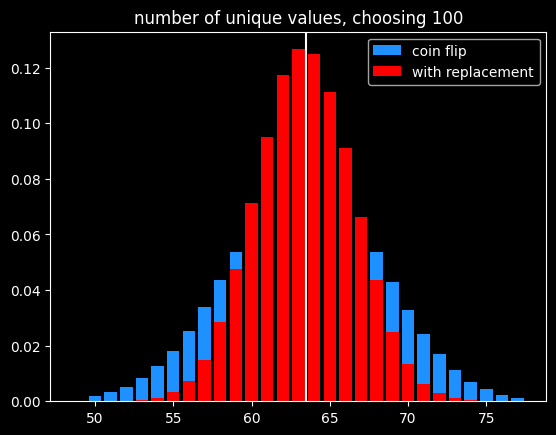
Of course, if the goal is to select exactly 63 items out of 100, the best way would be to randomly select 63 without replacement so there is no variation in the number of items selected.
A number's a number
Instead of selecting 100 times from 100 numbers, what if we selected a bajillion times from a bajillion numbers? To put it in math terms, what is $\lim\limits_{n\to\infty} (\frac{n-1}{n})^{n}$ ?
It turns out this is equal to $\frac{1}{e}$ ! Yeah, e! Your old buddy from calculus class. You know, the $e^{i\pi}$ guy?
As n goes to infinity, the probability of a number being selected is $1-\frac{1}{e} = .632$. This leads to a technique called bootstrapping, or ".632 selection" in machine learning (back to that in a minute).
Don't think of an answer
What are the chances that a number gets selected exactly once? Turns out, it's $\frac{1}{e}$, same as the chances of not getting selected! This was surprising enough to me to bother to work out the proof, given at the end.
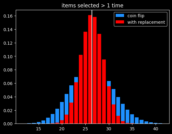
That means the chances of a number getting selected more than once is $1 - \frac{2}{e}$.
The breakdown:
- 1/e (36.8%) of numbers don't get selected
- 1/e (36.8%) get selected exactly once
- 1-2/e (26.4%) get selected 2+ times
As before, the variance in number of items picked 2+ times is much lower than flipping a coin that comes up heads 26.4% of the time:
Derangements
Say I'm handing out coats randomly after a party. What are the chances that nobody gets their own coat back?
This is called a derangement, and the probability is also 1/e. An almost correct way to think about this is the chance of each person not getting their own coat (or each coat not getting their own person, depending on your perspective) is $\frac{(x-1)}{x}$ and there are $x$ coats, so the chances of a derangement are $\frac{x-1}{x}^{x}$.
This is wrong because each round isn't independent. In the first case, we were doing selection with replacement, so a number being picked one round doesn't affect its probability of being picked next round. That's not the case here. Say we've got the numbers 1 thru 4. To make a derangement, the first selection can be 2, 3 or 4. The second selection can be 1, 3 or 4. But 3 or 4 might have been picked in the first selection and can't be chosen again. 2/3rds of the time, there will only be two options for the second selection, not three.
The long way 'round the mountain involves introducing a new mathematical function called the subfactorial, denoted as $!x$, which is equal to the integer closest to $\frac{x!}{e}$. $e$ gets in there because in the course of counting the number of possible derangements, a series is produced that converges to $1/e$.
The number of derangements for a set of size x is $!x$ and the number of permutations is $x!$, so the probability of a derangement as x gets big is $\frac{!x}{x!} = \frac{1}{e}$
What about the chances of only one person getting their coat back? It's also $\frac{1}{e}$, just like the chances of a number getting selected exactly once when drawing numbers with replacement. The number of fixed points -- number of people who get their own coat back -- follows a Poisson distribution with mean 1.
The second process seems very different from the first one. It is selection with replacement versus without replacement. But $e$ is sort of the horizon line of mathematics -- a lot of things tend towards it (or its inverse) in the distance.
Bootstrapping
Say we're working on a typical statistics/machine learning problem. We're given some training data where we already know the right answer, and we're trying to predict for future results. There are a ton of ways we could build a model. Which model will do the best on the unknown data, and how variable might the accuracy be?
Bootstrapping is a way to answer those questions. A good way to estimate how accurate a model will be in the future is to train it over and over with different random subsets of the training data, and see how accurate the model is on the data that was held out. That will give a range of accuracy scores which can be used to estimate how well the model will be on new inputs, where we don't know the answers ahead of time. If the model we're building has a small set of parameters we're fitting (like the coefficients in a linear regression), we can also estimate a range of plausible values for those parameters. If that range is really wide, it indicates a certain parameter isn't that important to the model, because it doesn't matter if it's big or small.
Bootstrapping is a way of answering those questions, using the process described before -- if we have x datapoints, pick x numbers without replacement x times. The ones that get selected at least once are used to train the models, and the ones that don't get selected are used to generate an estimate of accuracy on unseen data. We can do that over and over again and get different splits every time.
It's a fine way to split up the training data and the validation data to generate a range of plausible accuracy scores, but I couldn't find a good reason other than tradition for doing it that way. The 63.2/36.8 split isn't some magical value. Instead of having the numbers that weren't picked be the holdout group, we could instead leave out the numbers that were only picked once (also 1/e of the numbers), and train on the ones not selected or selected more than once. But picking 63% of values (or some other percentage) without replacement is the best way to do it, in my opinion.
The original paper doesn't give any statistical insight into why the choice was made, but a remark at the end says, "it is remarkably easy to implement on the computer", and notes the $4 cost of running the experiments on Stanford's IBM 370/168 mainframe. Maybe it's just the engineer in me, but it seems like a goofy way to do things, unless you actually want a variable number of items selected each run.
In the notebook, I showed that bootstrapping is about 40% slower than selection without replacement when using numpy's choice() function. However, the cost of selecting which items to use for training vs. testing should be insignificant compared to the cost of actually training the models using that train/test split.
A chance encounter
A quick proof of the chances of being selected exactly once.
Doing x selections with replacement, the chance of a number being chosen as the very first selection (and no other times) is
$\frac{1}{x} * \frac{x-1}{x}^{x-1}$
There are x possible positions for a number to be selected exactly once. Multiply the above by x, which cancels out 1/x. So the chances of a number being selected exactly once at any position is $(\frac{x-1}{x})^{x-1}$.
Let's try to find a number $q$ so that $\lim\limits_{x\to\infty} (\frac{x-1}{x})^{x-1} = e^{q}$.
Taking the log of both sides:
$q = \lim\limits_{x\to\infty} (x-1) * log(\frac{x-1}{x}) = \lim\limits_{x\to\infty} \frac{log(\frac{x-1}{x})}{1/(x-1)}$
Let
$f(x) = log(\frac{x-1}{x})$
and
$g(x) = \frac{1}{x-1}$
By L'Hopital's rule, $\lim\limits_{x\to\infty} \frac{f(x)}{g(x)} = \lim\limits_{x\to\infty}\frac{f'(x)}{g'(x)}$
The derivative of a log of a function is the derivative of the function divided by the function itself, so:
$f'(x) = \frac{d}{dx} log(\frac{x-1}{x}) = \frac{d}{dx} log(1 - \frac{1}{x}) = \frac{\frac{d}{dx}(1-\frac{1}{x})}{1-\frac{1}{x}} =\frac{\frac{1}{x^{2}}}{{1-\frac{1}{x}}} = \frac{1}{x^{2}-x} = \frac{1}{x(x-1)}$
and
$g'(x) = \frac{-1}{(x-1)^{2}}$
Canceling out (x-1) from both, $\frac{f'(x)}{g'(x)} = \frac{1}{x} * \frac{x-1}{-1} = -1 * \frac{x-1}{x}$.
So $q = \lim\limits_{x\to\infty} -1 * \frac{x-1}{x} = -1$
At the limit, the probability of being selected exactly once is $e^{-1} = \frac{1}{e}$
References/Further Reading
https://oeis.org/A068985
https://mathworld.wolfram.com/Derangement.html
Great explanation of how to calculate derangements using the inclusion-exclusion principle: https://www.themathdoctors.org/derangements-how-often-is-everything-wrong/
The bible of machine learning introduces bootstrapping, but no talk of why that selection process. https://trevorhastie.github.io/ISLR/ISLR%20Seventh%20Printing.pdf
The original bootstrap paper: https://sites.stat.washington.edu/courses/stat527/s14/readings/ann_stat1979.pdf
May 22, 2025
(notebook is available at github.com/csdurfee/ensemble_learning.)
Ensemble Learning
AI and machine learning systems are often used for classification. Is this email spam or not? Is this person a good credit risk or not? Is this a photo of a cat or not?
There are a lot of ways to build classifiers, and they all potentially have different strengths and weaknesses. It's natural to try combining multiple models together to produce better results than the individual models would.
Model A might be bad at classifying black cats but good at orange ones, model B might be bad at classifying orange cats but good at black ones, model C is OK at both. So if we average together the results of the three classifiers, or go with the majority opinion between them, the results might be better than the individual classifiers.
This is called an ensemble. Random forests and gradient boosting are two popular machine learning techniques that use ensembles of weak learners -- a large number of deliberately simple models that are all trained on different subsets of the data. This strategy can lead to systems that are more powerful than their individual components. While each little tree in a random forest is weak and prone to overfitting, the forest as a whole can be robust and give high quality predictions.
Majority Voting
We can also create ensembles of strong learners -- combining multiple powerful models together. Each individual model is powerful enough to do the entire classification on its own, but we hope to achieve higher accuracy by combining their results. The most common way to do that is with voting. Query several classifiers, and have the ensemble return the majority pick, or otherwise combine the results.
There are some characteristics of ensembles that seem pretty common sense [1]. The classifiers in the ensemble need to be diverse: as different as possible in the mistakes they make. If they all make the same mistakes, then there's no way for the ensemble to correct for that.
The more classification categories, the more classifiers are needed in the ensemble. However, in real world settings, there's usually a point where adding more classifiers doesn't improve the ensemble.
The Model
I like building really simple models. They can illustrate fundamental characteristics, and show what happens at the extremes.
So I created an extremely simple model of majority voting (see notebook). I'm generating a random list of 0's and 1's, indicating the ground truth of some binary classification problem. Then I make several copies of the ground truth and randomly flip x% of the bits. Each of those copies represent the responses from an individual classifier within the ensemble. Each fake classifier will have 100-x% accuracy. There's no correlation between the wrong answers that each classifier gives, because the changes were totally random.
For every pair of fake classifiers with 60% accuracy, they will both be right 60% * 60% = 36% of the time, and both wrong 40% * 40% = 16%. So they will agree 36% + 16% = 52% of the time at minimum.
That's different from the real world. Machine learning algorithms trained on the same data will make a lot of the same mistakes and get a lot of the same questions right. If there are outliers in the data, any classifier can overfit on them. And they're all going to find the same basic trends in the data. If there aren't a lot of good walrus pictures in the training data, every model is probably going to be bad at recognizing walruses. There's no way to make up for what isn't there.
Theory vs Reality
In the real world, there seem to be limits on how much an ensemble can improve classification. On paper, there are none, as the simulation shows.
What is the probability of the ensemble being wrong about a particular classification?
That's the probability that the majority of the classifiers predict 0, given that the true value is 1 (and vice versa). If each classifier is more likely to be right than wrong, as the number of classifiers goes to infinity, the probability of the majority of predictions being wrong goes to 0.
If each binary classifier has a probability > .5 of being right, we can make the ensemble arbitrarily precise if we add enough classifiers to the ensemble (assuming their errors are independent). We could grind the math using the normal approximation to get the exact number if need be.
Let's say each classifier is only right 50.5% of the time. We might have to add 100,000 of them to the ensemble, but we can make the error rate arbitrarily small.
Correlated errors ruin ensembles
The big difference between my experiment and reality is that the errors the fake classifiers make are totally uncorrelated with each other. I don't think that would ever happen in the real world.
The more the classifiers' wrong answers are correlated with each other, the less useful the ensemble becomes. If they are 100% correlated with each other, the ensemble will give the exact same results as the individual classifiers, right? An ensemble doesn't have to improve results.
To put it in human terms, the "wisdom of the crowd" comes from people in the crowd having wrong beliefs about uncorrelated things (and being right more often than not overall). If most people are wrong in the same way, there's no way to overcome that with volume.
My experience has been that different models tend to make the same mistakes, even if they're using very different AI/machine learning algorithms, and a lot of that is driven by weaknesses in the training data used.
For a more realistic scenario, I created fake classifiers with correlated answers, so that they agree with the ground truth 60% of the time, and with each other 82% of the time, instead of the minimum 52% of the time.
The Cohen kappa score is .64, on a scale from -1 to 1, so they aren't as correlated as they could be.
The simulation shows that if the responses are fairly strongly correlated with each other, there's a hard limit to how much the ensemble can improve things.
Even with 99 classifiers in the ensemble, the simulation only achieves an f1 score of .62. That's just a slight bump from the .60 achieved individually. There is no marginal value to adding more than 5 classifiers to the ensemble at this level of correlation.
Ensembles: The Rich Get Richer
I've seen voting ensembles suggested for especially tricky classification problems, where the accuracy of even the best models is pretty low. I haven't found that to be true, though, and the simulation backs that up. Ensembles are only going to give a significant boost for binary classification if the individual classifiers are significantly better than 50% accuracy.
The more accurate the individual classifiers, the bigger the boost from the ensemble. These numbers are for an ensemble of 3 classifiers (in the ideal case of no correlation between their responses):
| Classifier Accuracy |
Ensemble Accuracy |
| 55% |
57% |
| 60% |
65% |
| 70% |
78% |
| 80% |
90% |
Hard vs. soft voting
There are two different ways of doing majority voting, hard and soft. This choice can have an impact on how well an ensemble works, but I haven't seen a lot of guidance on when to use each.
Hard voting is where we convert the outputs of each binary classifier into a boolean yes/no, and go with the majority opinion. If there are an odd number of components and it's a binary classification, there's always going to be a clear winner. That's what I've been simulating so far.
Soft voting is where we combine the raw outputs of all the components, and then round the combined result to make the prediction. sklearn's documentation advises to use soft voting "for an ensemble of well-calibrated classifiers".
In the real world, binary classifiers don't return a nice, neat 0 or 1 value. They return some value between 0 or 1 indicating a relative level of confidence in the prediction, and we round that value to 0 or 1. A lot of models will never return a 0 or 1 -- for them, nothing is impossible, just extremely unlikely.
If a classifier returns .2, we can think of it as the model giving a 20% chance that the answer is 1 and an 80% chance it's 0. That's not really true, but the big idea is that there's potentially additional context that we're throwing away by rounding the individual results.
For instance, say the raw results are [.3,.4,.9]. With hard voting, these would get rounded to [0,0,1], so it would return 0. With soft voting, it would take the average of [.3,.4,.9], which is .53, which rounds to 1. So the two methods can return different answers.
To emulate the soft voting case, I flipped a percentage of the bits, as before. Then I replaced every 0 with a number chosen randomly from the uniform distribution from [0,.5] and every 1 with a sample from [.5,1]. The values will still round to what they did before, but there's additional noise on top.
In this simulation (3 classifiers), the soft voting ensemble gives less of a boost than the hard voting ensemble -- about half the benefits. As with hard voting, the more accurate the individual classifiers are, the bigger the boost the ensemble gives.
| Classifier Accuracy |
Ensemble Accuracy |
| 55% |
56% |
| 60% |
62% |
| 70% |
74% |
| 80% |
85% |
Discussion
Let's say a classifier returns .21573 and I round that down to 0. How much of the .21573 that got lost was noise, and how much was signal? If a classification task is truly binary, it could be all noise. Let's say we're classifying numbers as odd or even. Those are unambiguous categories, so a perfect classifier should always return exactly 0 or 1. It shouldn't say that three is odd, with 90% confidence. In that case, it clearly means the classifier is 10% wrong. There's no good reason for uncertainty.
On the other hand, say we're classifying whether photos contain a cat or not. What if a cat is wearing a walrus costume in one of the photos? Shouldn't the classifier return a value greater than 0 for the possibility of it not being a cat, even if there really is a cat in the photo? Isn't it somehow less cat-like than another photo where it's not wearing a walrus costume? In this case, the .21573 at least partially represents signal, doesn't it? It's saying "this is pretty cat-like, but not as cat-like as another photo that scored .0001".
When I'm adding noise to emulate the soft voting case, is that fair? A different way of fuzzing the numbers (selecting the noise from a non-uniform distribution, for instance) might reduce the gap in performance between hard and soft voting ensembles, and it would probably be more realistic. But the point of a model like this is to show the extremes -- it's possible that hard voting will give better results than soft voting, so it's worth testing.
Big Takeaways
- Ensembles aren't magic; they can only improve things significantly if the underlying classifiers are diverse and fairly accurate.
- Hard and soft voting aren't interchangeable. If there's a lot of random noise in the responses, hard voting is probably a better option, otherwise soft voting is probably better. It's definitely worth testing both options when building an ensemble.
- Anyone thinking of using an ensemble should look at the amount of correlation between the responses from different classifiers. If the classifiers are all making basically the same mistakes, an ensemble won't help regardless of hard vs. soft voting. If models with very different architectures are failing in the same ways, that could be a weakness in the training data that can't be fixed by an ensemble.
References
[1] Bonab, Hamed; Can, Fazli (2017). "Less is More: A Comprehensive Framework for the Number of Components of Ensemble Classifiers". arXiv:1709.02925
Tsymbal, A., Pechenizkiy, M., & Cunningham, P. (2005). Diversity in search strategies for ensemble feature selection. Information Fusion, 6(1), 83–98. doi:10.1016/j.inffus.2004.04.003